
| From | To | Coefficient |
|---|---|---|
| intercept | open_data | -3 |
| rigour | open_data | 0.1 |
| field | open_data | 1, 5 |
| intercept | published | -1 |
| novelty | published | 1 |
| rigour | published | 2 |
| open_data | published | 8 |
| intercept | data_reuse | -1 |
| open_data | data_reuse | 2 |
| novelty | data_reuse | 1 |
| intercept | reproducibility | 1 |
| open_data | reproducibility | 0.4 |
| rigour | reproducibility | 1 |
| intercept | citations | -1 |
| novelty | citations | 2 |
| rigour | citations | 2 |
| published | citations | 2 |
| data_reuse | citations | 2 |
| field | citations | 10, 20 |
| sigma | none | 1 |
Causality in science studies
Introduction
Causal questions are pervasive in science studies: what are the effects of peer review on the quality of publications (Goodman et al. 1994)? What is the influence of mentorship on protegees success (Malmgren, Ottino, and Nunes Amaral 2010)? Do incentives to share research data lead to higher rates of data sharing (Woods and Pinfield 2022)? Yet, answers to such questions are rarely causal. Often, researchers investigate causal questions, but fail to employ adequate methods to make causal claims. As an example, there is a burgeoning literature investigating whether publishing Open Access leads to more citations. While the observational evidence seems to suggest such an effect, few studies use methods that would permit causal claims (Klebel et al. 2023). Most scientists acknowledge that we should be “thinking clearly about correlation and causation” (Rohrer 2018), but the implications of causal considerations are often ignored. Similar concerns were raised in the context of biases in science, such as gender bias (Traag and Waltman 2022).
Uncovering causal effects is a challenge shared by many scientific fields. There are large methodological differences between fields, also with regards to inferring causality. Some fields are experimental, while others are observational. Some are historical, examining a single history, while others are contemporary, where observations can be repeated. Some fields already have a long tradition with causal inference, while other fields have paid less attention to causal inference. We believe that science studies, regardless of whether that is scientometrics, science of science, science and technology studies, or sociology of science, have paid relatively little attention to questions of causality, with some notable exceptions (e.g., Aagaard and Schneider 2017; Gläser and Laudel 2016).
We here provide an introduction to causal inference for science studies. Multiple introductions to structural causal modelling of varying complexity already exist (Rohrer 2018; Arif and MacNeil 2023; Elwert 2013). Dong et al. (2022) introduce matching strategies to information science. We believe it is beneficial to introduce causal thinking using familiar examples from science studies, making it easier for researchers in this area to learn about causal approaches. We avoid technicalities, so that the core ideas can be understood even with little background in statistics.
The fundamental problem
The fundamental problem in causal inference is that we never have the answer to the “what-if” question. For instance, suppose that a professor received tenure. We can observe her publications when she received tenure. Would she also have received tenure, if she had not published that one paper in a high-impact journal? We cannot simply observe the answer, since that situation did not materialize: she in fact did publish that paper in a high-impact journal, and in fact did receive tenure. The so-called counterfactual scenario, where she did not publish that paper and received tenure (or not), is unobservable. This unobservable counterfactual scenario is the fundamental problem.
Experiments are often helpful in getting causal answers. By controlling the exact conditions, and only actively varying one condition, we can recreate counterfactual scenarios, at least on average, assuming conditions are properly randomised. There are also some experimental studies in science studies, for instance studying the effect of randomly tweeting about a paper or not (Luc et al. 2021; Davis 2020), making papers randomly openly available (Davis et al. 2008), or studying affiliation effects by experimentally comparing double-anonymous peer review with single-anonymous peer review (Tomkins, Zhang, and Heavlin 2017). However, there are many questions that do not allow for an experimental setup. For example, randomising scholars’ career age or research field is impossible. But even in experimental settings there are limitations to causal inference. For instance, non-compliance in experimental settings might present difficulties (Balke and Pearl 2012), such as certain types of reviewers being more likely to try to identify authors in a double-anonymous peer review experiment. Additionally, scholars might be interested in identifying mediating factors when running experiments, which further complicates identifying causality (Rohrer et al. 2022). In other words, causal inference presents a continuum of challenges, where experimental settings are typically easiest for identifying causal effects—but certainly no panacea—and observational settings are more challenging—but certainly not impossible.
In this paper we introduce a particular view on causal inference, namely that of structural causal models (Pearl 2009). This is a relatively straightforward approach to causal inference with a clear visual representation of causality. It should allow researchers to reason and discuss about their causal thinking more easily. In the next section, we explain structural causal models in more detail. We then cover some case studies based on simulated data to illustrate how causal estimates can be obtained in practice. We close with a broader discussion on causality.
Causal inference - a brief introduction
Structural causal models focus, as the name suggests, on the structure of causality, not on the exact details. That is, structural causal models are only concerned with whether a certain factor is causally affected by another factor, not whether that effect is linear, exponential, or an “interaction” with some other effects. Such structural models can be represented by simple causal diagrams. This graphical approach makes it relatively easy to discuss about causal models and assumptions, because it does not necessarily involve complicated mathematics.
Sometimes, assumptions about specific functional dependencies can be made, and this might help causal inference. For instance, a well-known general causal inference strategy is called “difference-in-difference”. A key assumption in that strategy is something called “parallel trends”. Not having to deal with such details simplifies the approach and makes it easier to understand the core concepts. But sometimes it also simplifies too much. We can always make stronger assumptions, and sometimes, these stronger assumptions allow us to draw stronger conclusions. But without assumptions, we cannot conclude anything.
The overall approach to causal inference using structural causal models would be the following:
- Assume a certain structural causal model.
- Use the assumed structural causal to understand how to identify causal effects.
- Identified effects can be interpreted causally under the assumed structural causal model.
Whatever structural causal model we construct, it will always be an assumption. Constructing such a structural causal model can be based on domain expertise and prior literature in the area. Whether a structural causal is realistic or not might be debated. This is a good thing, because by making causal assumptions explicit, we can clarify the discussion, and perhaps advance our common understanding. We cannot always use empirical observations to discern between different structural causal models. That is, different structural causal models can have the same observable implications, and so no observations would help discern between them. However, there might also be observable implications that do differ between different structural causal models. We can then put the two (or more) proposed theoretical structural causal models to the test, using empirical evidence to decide which structural causal model is incorrect. Note the emphasis on incorrect: we cannot say that a structural causal model is correct, but we can say that a structural causal model is incorrect, if it is inconsistent with the observations. In summary, if we propose a certain structural causal model to try to identify a causal effect, we should make sure that its observable implications are at least consistent with the empirical evidence we have.
Nonetheless, any structural causal model always remains a simplification of reality, and is usually designed for a specific causal question. For example, a structural causal model of the entire academic system, containing each and every detail about potential effects, is overly detailed and likely not useful for the majority of empirical studies. For most studies, a simpler structural causal model is probably more productive. In some cases, problems of causal identification might emerge in simple structural causal models, and are not heavily dependent on specific details. That is, adding more nuance to a structural causal model will not necessarily solve a problem that was identified in a simpler structural causal model. However, sometimes problems might only become apparent with more complex structural causal models, and additional nuance might reveal that identifying a causal effect is more challenging. We encounter and discuss this in some examples later.
The main challenge then is to use a given structural causal model to identify a causal effect: what factors should be controlled for and, equally important, what factors should not be controlled for? We introduce an answer to that question in the next subsection. The introduction we provide here only covers the basics. We explicitly provide an introduction that is as simple as possible, in order to be understandable to a broad audience. Our introduction covers many typical situations that can be encountered, but there are other cases that cannot be understood without using a more formal logic known as do-calculus (Pearl 2009). Beyond existing introductions to causal inference, typically covering specific fields (Rohrer 2018; Arif and MacNeil 2023; Hünermund and Bareinboim 2023; Deffner, Rohrer, and McElreath 2022), there are also comprehensive text-books (Huntington-Klein 2021; Cunningham 2021; Pearl 2009), that provide much more detail and explanation than we can provide here.
To provide an introduction useful to readers and scholars in science studies, we consider the case of Open Science, a movement and practice of making research processes more transparent (Fecher and Friesike 2014). Many studies have been conducted on the potential impacts Open Science might have on academia, society, and the economy (Klebel et al. 2023; Tennant et al. 2016). However, studies on specific types of Open Science impact, such as those on the Open Access citation advantage, often lack a clear understanding of causal pathways and thus fail to develop a meaningful strategy for estimating causal effects. Our introduction shows how causal inference could be leveraged to improve these and similar studies.
Introducing DAGs

It is convenient to represent a structural causal model using a directed acyclic graph (DAG). A DAG is a directed graph (sometimes called a network) where the nodes (sometimes called vertices) represent variables, and the links (sometimes called edges) represent causal effects. A DAG is acyclic, meaning that there cannot be directed cycles, so that if \(X \rightarrow Z \rightarrow Y\), there cannot be a link \(Y \rightarrow X\) (or \(Y \rightarrow Z\) or \(Z \rightarrow X\)). If there is a \(X \rightarrow Y\), it means that \(Y\) directly depends on \(X\), that is, \(Y\) is a function of \(X\). We do not specify what function exactly, so it can be a linear function, an exponential function, or any complicated type of function. Interactions between variables, moderators, hurdles, or any other type of functional specification are not indicated separately, and all can be part of the function.
The variables that influence \(Y\) directly, i.e. for which there is a link from that variable to \(Y\), are called the parents of \(Y\). If any of the parents of \(Y\) change, \(Y\) will also change1. If any parents of the parents change, i.e. variables that are further upstream, \(Y\) will also change. Hence, if there are any paths from \(X\) to \(Y\), possibly through other variables \(Z\), i.e. \(X \rightarrow Z \rightarrow Y\), the variable \(X\) has a causal effect on \(Y\).
Throughout this introduction, we work with a single example DAG on Open Science (see Figure 1). In this DAG, Novelty and Rigour are both assumed to affect the number of Citations and whether something will be Published or not. Here, we use Published to refer to a journal publication, but research can also be made available in different ways, for example as preprints or working papers. Preprints or working papers can also be considered published, but for the sake of simplicity we use the term Published to refer to journal publications only. Unlike Novelty, Rigour influences whether data is made available openly: scholars that are doing more rigorous research may be more likely to share their data openly. Unlike Rigour, Novelty affects Data reuse; data from a rigorous study that did not introduce anything new may be less likely to be reused by other researchers. If data is reused, the original study might be cited again, so Data reuse is assumed to affect Citations. In some cases, Open data will be mandated by a journal, and so whether something will be Published may also depend on Open data. Whether something is Reproducible is assumed to be affected by the Rigour of the study, and also by Open data itself: studies that share data might lead scholars to double check all their results to make sure they align exactly with the shared data. Finally, Citations are also influenced by the Field of study (some fields are more citation intensive), as is Open data (data sharing culture is not the same across fields).
As explained earlier, this DAG is a simplification, and we can debate whether it should be changed in some way. However, the DAG is consistent with most results from the literature, although there is typically also disagreement within the literature itself. This DAG is constructed without one particular causal question in mind. Instead, we illustrate all the necessary concepts using this example, and use this DAG for multiple possible causal questions. For a particular study, it might be best to construct a particular DAG for the specific causal question. A reasonable starting point for constructing a DAG for a particular causal question of \(X\) on \(Y\) might be the following: (1) consider all factors that affect and are affected by \(X\) and/or \(Y\); (2) consider how these factors are causally related between each other. There might be additional relevant considerations, but it should provide a reasonable simplification to start with.
A useful tool for working with DAGs is called dagitty, which is available from the website http://dagitty.net, which also contains many useful pointers to additional introductions and tutorials.
Using DAGs to identify causal effects
Most scholars will be acquainted with problems of confounding effects, and that we somehow need to “control” for confounding effects. But there are also other factors besides confounders. Most scholars will also be acquainted with mediating factors, i.e. mediators. Fewer scholars will be acquainted with colliding factors, i.e. colliders. Controlling for a collider often leads to incorrect causal inferences. Hence, the question of what variables to control for is more complicated than just controlling for confounders. In particular, colliders raise the question what we should not control for. In this section, we use DAGs to understand which factors we should control for, and which factors we should not control for.
We are interested in the causal effect of one variable \(X\) on another variable \(Y\). As the popular adage goes, correlation does not imply causation. That is, \(X\) and \(Y\) might be correlated, even if \(X\) does not affect \(Y\). For instance, in Figure 1 Reproducibility and Published are correlated because both are affected by Open data, but Reproducibility does not have any causal effect on Published or vice versa.
Paths in DAGs
In DAGs, we think of correlation and causation in terms of paths between variables. In a graph, a path between two nodes consists of a series of connected nodes. That is, we can move from one node to another across the links between the nodes to reach another part of the graph. For example, in Figure 1 we can move from Novelty to Data reuse to Citations. In this example, the path follows the direction of the links. Paths that follow the direction of the links resemble the flow of causality, and we refer to them as causal paths. That is, Novelty affects Data reuse, which in turn affects Citations. This is an indirect causal effect of Novelty on Citations, mediated by Data reuse. There is another indirect causal effect of Novelty on Citations, mediated by Published. In addition, there is also a link directly from Novelty to Citations, which represents a direct causal effect. The combination of the two indirect effects and the direct effect is known as the total causal effect.
In addition, there are also paths that do not follow the direction of the links. This can be most easily done by simply ignoring the directions, and also allowing to traverse links upstream, so to speak. There is then a path between Open data and Citations through Field. There is not a single direction that we follow, and the path looks like Open data \(\leftarrow\) Field \(\rightarrow\) Citations. Paths that do not follow a single direction do not represent a causal effect, and we refer to them as non-causal paths.
The key insight is that two variables that are connected through certain paths are correlated, even if they are not connected through any causal paths. We discern two types of paths. One type of path, through which two variables are correlated, is called an open path. Another type of path, through which two variables are not correlated, is called a closed path. If there are no open paths between two variables, the two are not correlated. Both causal paths and non-causal paths can be open or closed. Indeed, if there is a non-causal path that is open, two variables are correlated, but this “correlation does not imply causation”.
Formalising this slightly, two variables \(X\) and \(Y\) are correlated if there is an open path between \(X\) and \(Y\). If there are no open paths between \(X\) and \(Y\), they are not correlated2. We can identify a causal effect of \(X\) on \(Y\) by closing all non-causal paths between \(X\) and \(Y\) and by opening all causal paths from \(X\) to \(Y\). Whether a path is open or closed depends on the types of variables on a path, and whether those variables are conditioned on. We explain this in more detail below, and provide a visual summary of the explanation in Figure 2.

As explained, all paths between \(X\) and \(Y\) need to be considered, regardless of their direction. That is, \(X \rightarrow Z \rightarrow Y\) is a path that we should consider, but also \(X \leftarrow Z \rightarrow Y\) and \(X \rightarrow Z \leftarrow Y\). Going back to the paths we considered earlier: if we are interested in the causal effect of Open data on Citations, there is a directed, causal path from Open data to Data reuse to Citations, but there is also a non-causal path between Open data and Citations that runs through Field.3
We call a path open when all the nodes, i.e. variables, on the path are open. If there is a single closed variable on a path, the entire path is closed. You can think of this as a sort of information flow: if all nodes are open, information can flow through, but a single closed node blocks the flow of information. We can change whether a variable should be considered open or closed by conditioning on it. By closing a variable, we can therefore close a path. By opening a variable, we can potentially open a path, unless the path is still closed by another variable.
There are many ways in which we can condition on a variable. A common approach in quantitative analysis is to include such a variable in a regression analysis. But another way is to analyse effects separately for various categories of some variable. For example, we can condition on Field by performing an analysis for each field separately. This can be thought of as comparing cases only within these categories. Other approaches include for example so-called matching procedures. When matching cases on a certain variable, we only compare cases which are the same (or similar) on that variable. Finally, in science studies, indicators are frequently “normalised”, especially citation indicators (Waltman and Eck 2019), which amounts to conditioning on the variables used for the normalisation.
Confounders, colliders and mediators
We can discern three types of variables: a confounder, a collider and a mediator. Whether a variable \(Z\) is a confounder, a collider or a mediator depends on how \(Z\) is connected on a path between \(X\) and \(Y\). Below we consider each type of variable in more detail.
The first type of variable that we consider is a confounder. A confounder \(Z\) is always connected like \(X \leftarrow Z \rightarrow Y\). Here \(Z\) is the common cause for both \(X\) and \(Y\). A confounder is open when not conditioned on. If we condition on a confounder, it is closed. Usually, we want to close paths with confounders, as the paths do not represent a causal effect. For example, in Figure 1, Field plays the role of a confounder on the path between Open data and Citations. That path is open; we can close it by conditioning on Field.
The second type of variable that we consider is a collider. A collider \(Z\) is always connected like \(X \rightarrow Z \leftarrow Y\). Here \(Z\) is affected by both \(X\) and \(Y\). A collider is closed when not conditioned on. If we condition on a collider, it is opened. Usually, we want to keep paths with a collider closed, as the paths do not represent a causal effect. For example, in Figure 1, Published plays the role of a collider on the path between Rigour and Novelty. That path is closed; we can open it by conditioning on Published.
Finally, the third type of variable that we consider is a mediator. A mediator \(Z\) is always connected like \(X \rightarrow Z \rightarrow Y\). Here, \(Z\) is affected by \(X\) and in turn \(Z\) affects \(Y\). Indirectly, namely through \(Z\), \(X\) affects \(Y\). A mediator is open when not conditioned on. If we condition on a mediator, it is closed. Usually, we want to keep paths with mediators open, as the paths represent a causal effect. However, it might be that we are interested in the direct effect of \(X\) on \(Y\), instead of the total effect of \(X\) on \(Y\). By controlling for a mediator \(Z\) we can close the indirect path \(X \rightarrow Z \rightarrow Y\), and estimate the direct path \(X \rightarrow Y\) (assuming there are no other indirect paths left). For example, in Figure 1, Open data is a mediator between Rigour and Reproducibility. That path is open; we can close it by conditioning on Open data. This is relevant if we try to identify the direct causal effect of Rigour on Reproducibility.
Note that the same variable can play different roles in different paths. For example, in Figure 1, Open data plays the role of a confounder in the path Reproducibility \(\leftarrow\) Open data \(\rightarrow\) Data Reuse \(\rightarrow\) Citations. At the same time, Open data plays the role of a collider in the path Reproducibility \(\leftarrow\) Rigour \(\rightarrow\) Open data \(\leftarrow\) Field \(\rightarrow\) Citations. The former path is open, while the latter path is closed. If we are interested in the causal effect, both paths should be closed, since neither represents a causal effect. However, if we condition on Open data, we close the path where Open data is a confounder, while we open the path where Open data is a collider. Hence, we cannot close both paths by conditioning on Open data. If we cannot condition on other variables, for example because we did not collect such variables for a study, we have no way of identifying the causal effect4 of Reproducibility on Citations.
Case studies
In this section, we apply the concepts introduced above to potential research questions, demonstrating how to estimate causal effects. We show how a researcher can use a hypothesised causal model of the phenomenon under study to estimate causal effects. We use the DAG introduced earlier (Figure 1) to illustrate our estimation strategies.
For the purposes of these hypothetical examples, we simulate data according to the DAG in Figure 1. As explained, a DAG only specifies that a variable is affected by another variable, but it does not specify how. For simulating data, we do need to specify the model in more detail. In particular, we sample Field uniformly from two fields; we sample Rigour and Novelty from standard normal distributions (i.e. with a mean of 0 and a standard deviation of 1); we sample Open data and Published from Bernoulli distributions (i.e. Yes or No); and we sample Data reuse, Reproducibility and Citations again from standard normal distributions. The effects of some variables on other variables are represented by simple linear equations (using a logistic specification for the Bernoulli distributions), with particular coefficients for the effects (see Table 1). These distributions are not necessarily realistic. Yet, our aim is not to provide a realistic simulation, but to illustrate how causal inference can be applied. Relying on standard normal distributions and linear equations simplifies the simulation model and the analyses of the simulated data.
Regression analysis is the common workhorse of quantitative analysis, also in science studies. We use regression analysis to illustrate how a researcher might analyse their data to provide causal estimates5. Of course, more complex analytical approaches, such as Bayesian models or non-linear models can also be used. Such models might have great scientific, philosophical, or practical benefits, but they are certainly no prerequisite for sound causal inference. Moreover, having complex models is no substitute for sound causal inference, and wrong causal conclusions can still be drawn from complex models. From that point of view, using simpler methods while paying proper attention to causality might be preferred over using complex methods while ignoring issues of causality.
The effect of Rigour on Reproducibility
To provide a first impression of the simulated data, and some intuition of how we can estimate causal effects, we first analyse the effects of Rigour and Open data on Reproducibility (see Figure 3). Rigour and Reproducibility are clearly positively correlated: higher Rigour is associated with higher Reproducibility. We also see that the overall level of reproducibility tends to be higher if there is Open Data.
Show the code
df %>%
  mutate(open_data = case_when(!open_data ~ "Closed data",
                               TRUE ~ "Open data")) %>%
  ggplot(aes(rigour, reproducibility, color = open_data)) +
  geom_point(alpha = .4) +
  geom_smooth(method = "lm") +
  colorspace::scale_color_discrete_diverging(palette = "Tropic") +
  labs(x = "Rigour", y = "Reproducibility", color = NULL) +
  theme(legend.position = "top") +
  guides(colour = guide_legend(override.aes = list(fill = NA),
                               reverse = TRUE))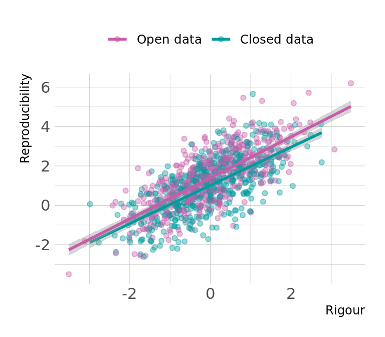
Following our model (Figure 1), Rigour and Open data are the only variables influencing Reproducibility. Let us consider the total causal effect of Rigour on Reproducibility. There are several paths between Rigour and Reproducibility, some causal, some non-causal. The model shows two causal paths: a direct effect Rigour \(\rightarrow\) Reproducibility and an indirect effect Rigour \(\rightarrow\) Open data \(\rightarrow\) Reproducibility, where the effect is mediated by Open data. The non-causal paths are more convoluted: all run through Citations and/or Published, with both variables acting as colliders on these paths. The non-causal paths are hence all closed, unless we condition on any of the colliders.
Since the causal paths are open, and the non-causal paths are closed, we do not have to control for anything. We can estimate the total causal effect of Rigour on Reproducibility simply with a regression of the form
\[\text{Reproducibility} \sim \text{Rigour}\]
Show the code
# compute the theoretical effect of rigour on reproducibility
field1 <- function(x) x * plogis(get_coefs("intercept", "open_data") + get_coefs("rigour", "open_data") * x + get_coefs("field", "open_data")[[1]]) * dnorm(x)
field2 <- function(x) x * plogis(get_coefs("intercept", "open_data") + get_coefs("rigour", "open_data") * x + get_coefs("field", "open_data")[[2]]) * dnorm(x)

rigour_effect_on_reproducibility <- get_coefs("rigour", "reproducibility") + get_coefs("open_data", "reproducibility") * mean(c(integrate(field1, -Inf, Inf)$value, integrate(field2, -Inf, Inf)$value))

m_rigour_reprod <- lm(reproducibility ~ rigour, data = df)
# summary(m_rigour_reprod)
Since we simulated the data, we can calculate the “true” causal effect, which in this case is 1 (see Appendix 5 for details). We can hence validate our regression approach and see if it is capable of correctly inferring the true causal effect. Figure 4 shows that the regression approach is capable of retrieving the correct result. We deliberately chose a moderate sample size of 1000 for our simulation. Point estimates derived from the simulated data thus only approximate the theoretical values.
Show the code
model_coefs <- tidy(m_rigour_reprod, conf.int = TRUE) %>%
    mutate(term = case_match(term,
                           "rigour" ~ "Rigour"))

# plot
text_label <- tibble(x = c(rigour_effect_on_reproducibility),
                     y = c("Rigour"),
                     label = "True effect")

pal <- colorspace::diverge_hcl(palette = "Tropic", n = 2)
highlight_col <- pal[2]
base_col <- pal[1]

model_coefs %>%
  filter(term != "(Intercept)") %>%
  ggplot() +
  ggdist::geom_pointinterval(aes(estimate, term,
                                 xmin = conf.low, xmax = conf.high), size = 8,
                             colour = base_col) +
  # annotate("point", y = "Open Data", x = open_data_effect_on_reproducibility,
  #          colour = highlight_col, size = 8, shape = "|") +
  annotate("point", y = "Rigour", x = rigour_effect_on_reproducibility,
           colour = highlight_col, size = 8, shape = "|") +
  scale_x_continuous(breaks = c(1, 2), labels = c(1, 2)) +
  geom_text_repel(data = text_label, aes(x = x, y = y, label = label),
                  nudge_x = .15, nudge_y = .4, colour = highlight_col) +
  labs(y = NULL, x = "Model estimate") +
  theme_ipsum_rc(grid = "XY") +
  coord_cartesian(xlim = c(1, 2))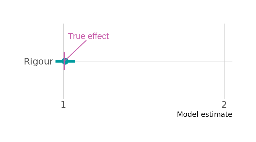
The example serves to highlight two points. First, it can be helpful to plot the data to gain an intuitive understanding of what the assumed relationship looks like. Second, sound causal inference does not necessarily involve controlling for many variables. In some cases, a simple regression might be all that is needed. Not all causal effects are equally straightforward to measure, as the next examples show.
The effect of Open data on Citations
Suppose we are interested in the total causal effect of Open data on Citations. Previous research on the topic indicates that articles sharing data tend to receive more citations (Piwowar, Day, and Fridsma 2007; Piwowar and Vision 2013; Kwon and Motohashi 2021). According to our model (Figure 1), there are multiple pathways from Open data to Citations. To estimate the causal effect, we need to make sure that all causal paths are open, and all non-causal paths are closed (see panel A in Figure 5).
There are two causal paths, both indirect: one mediated by Data reuse and one mediated by Published. To estimate the total causal effect of Open data on Citations we hence should not control for either Data reuse or Published. In contrast, typical approaches in scientometrics examine only the literature published in journals and hence implicitly condition on Published. This implicit conditioning closes the causal path, and thus biases our estimate of the total causal effect of Open data on Citations.
The non-causal paths pass through Rigour, Field or Reproducibility. On all paths passing through Rigour, it acts as a confounder, and we can hence close all these non-causal paths by controlling for Rigour. There is only one non-causal path where Field is acting as a confounder, and we can close it by conditioning on it. The remaining paths pass through Reproducibility, and it acts as a collider on all those paths. Hence, those paths are already closed. In summary, we should control for Rigour and Field.
The final regression model to estimate the causal effect of Open data on Citations is thus as follows:
\[ \textrm{Citations} \sim \textrm{Open data} + \textrm{Field} + \textrm{Rigour} \]
Show the code
# Calculate the theoretically expected causal effect of open_data on citations
theoretical_effect_OD_on_published <- momentsLogitnorm(
  mu = get_coefs("intercept", "published") + get_coefs("open_data", "published"),
  sigma = sigma
) - momentsLogitnorm(mu = get_coefs("intercept", "published"),
                     sigma = sigma)

theoretical_effect_OD_on_published <- theoretical_effect_OD_on_published["mean"]

open_data_effect_on_citations <- get_coefs("open_data", "data_reuse") * get_coefs("data_reuse", "citations") +
                                theoretical_effect_OD_on_published * get_coefs("published", "citations")

# # theoretical effect
# open_data_effect_on_citations

m_od_citations <- lm(citations ~ open_data + field + rigour, data = df)
Show the code
# plot
model_coefs <- tidy(m_od_citations, conf.int = TRUE) %>%
  mutate(term = case_match(term,
                           "rigour" ~ "Rigour",
                           "open_dataTRUE" ~ "Open Data",
                           "field" ~ "Field"))

text_label <- tibble(x = open_data_effect_on_citations,
                     y = "Open Data",
                     label = "True effect")

p <- model_coefs %>%
  filter(term != "(Intercept)") %>%
  ggplot() +
  ggdist::geom_pointinterval(aes(estimate, term,
                                 xmin = conf.low, xmax = conf.high), size = 5,
                             colour = base_col) +
  annotate("point", y = "Open Data", x = open_data_effect_on_citations,
           colour = highlight_col, size = 8, shape = "|") +
  geom_text_repel(data = text_label, aes(x = x, y = y, label = label),
                  nudge_x = 1.5, nudge_y = .3, colour = highlight_col, size = 3) +
  labs(y = NULL, x = "Model estimate") +
  theme_ipsum_rc(grid = "YX", base_size = 10, axis_title_size = 10 ) +
  theme(plot.margin = margin(10, 10, 10, 10))

# plot both figures
dag_grob <- image_read_pdf(here("causal_intro/article/figures/model_open_data_citations.pdf")) %>%
  as.grob()

design <- "
  111##
  11122
  11122
  11122
  111##
"

wrap_elements(dag_grob) + p +
  plot_layout(design = design) +
  plot_annotation(tag_levels = "A") &
  theme(plot.tag = element_text(size = 15))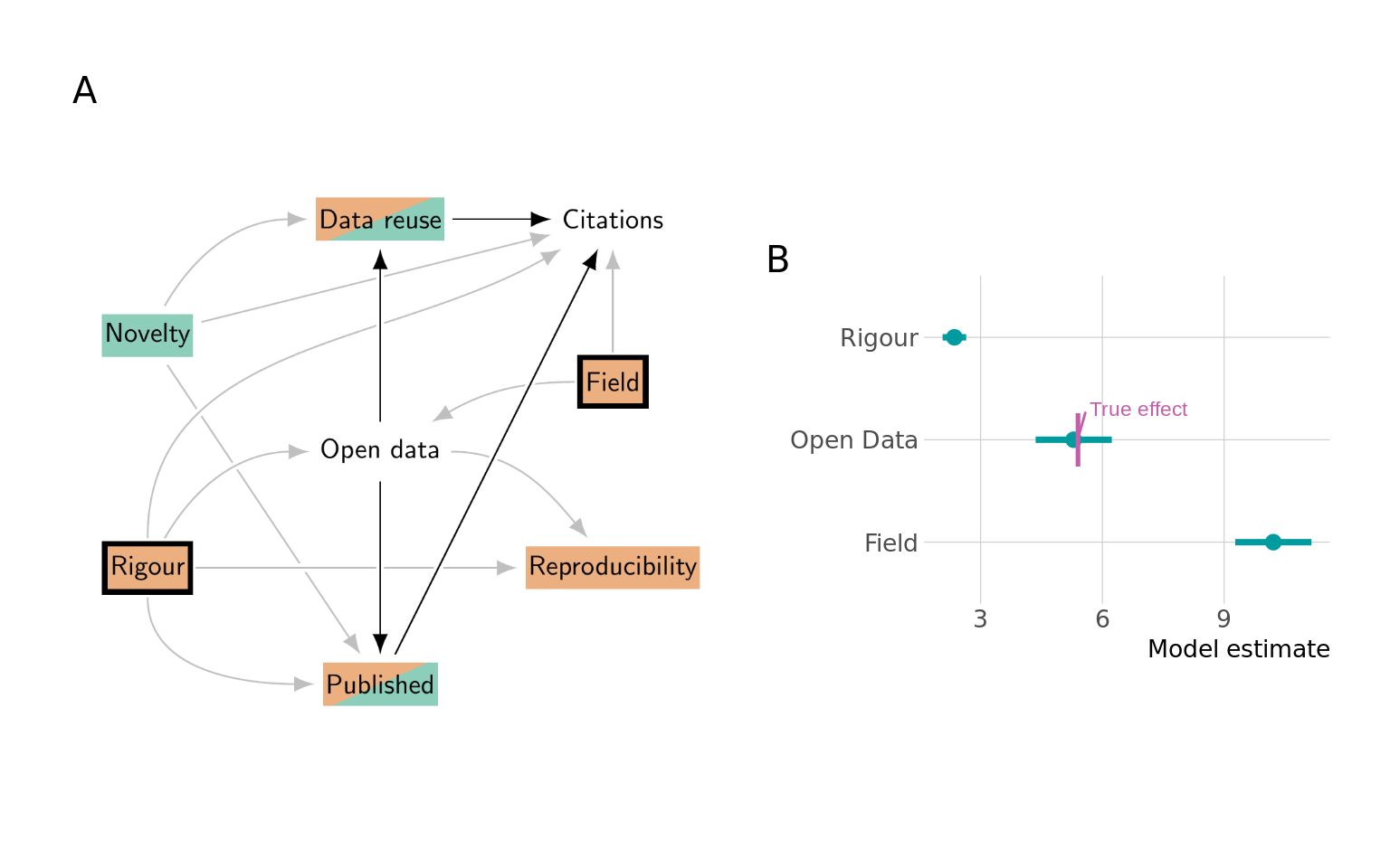
Figure 5 (B) shows the effect estimates from our regression, alongside the true effect of Open data on Citations, which is 5.39. We can see that our model is indeed able to estimate the causal effect of Open data on Citations.
This example highlights key components of causal inference: controlling for confounders (Rigour and Field), not controlling for mediators (Data reuse and Published), and not controlling for colliders (Reproducibility). This shows that constructing an appropriate DAG is crucial when aiming to draw causal conclusions. Without making assumptions explicit via a DAG, it would be unclear which variables should be controlled for and which not.
Some researchers might be tempted to defer the decision of what variables to control for to the data (for example via stepwise regression) or not make any decision at all by simply including all available variables (an approach termed “causal salad” by McElreath (2020)). However, neither approach is able to correctly identify the correct variables to control for. Stepwise regression would in this case suggest including the mediating variables (and even excluding Open data), leading to wrong causal conclusions (see Appendix 7). Including all variables could similarly lead the researcher to conclude that Open data has no effect on Citations (see Appendix 8).
The example highlights that relatively simple DAGs are often sufficient to uncover limitations to identifying causal effects. For instance, if we had not measured Field, controlling for it and identifying the causal effect would become impossible. In that case, it is irrelevant whether there are any other confounding effects between Citations and Open data, since those effects do not alleviate the problem of being unable to control for Field.
The effect of Open data on Reproducibility
Suppose we are interested in the causal effect of Open data on Reproducibility. Such an effect is often assumed in debates on how to increase the reproducibility across the scholarly literature (Molloy 2011). The empirical evidence so far is less convincing (Nuijten et al. 2017; Hardwicke et al. 2018, 2021; Nosek et al. 2022, 721). In our DAG in Figure 1, we assume there is a causal effect of Open data on Reproducibility. The causal effect is direct, there is no indirect effect of Open data on Reproducibility. Although the DAG does not specify these parametric assumptions, in our simulation, the effect is positive.
Conditioning on a collider may bias estimates
Many bibliometric databases predominantly cover research published in journals or conferences, which result from a clear selection process. Science studies frequently relies on such bibliometric databases for analysis. By only considering the literature published in journals, we (implicitly) condition on Published. On the path Open data \(\rightarrow\) Published \(\leftarrow\) Rigour \(\rightarrow\) Reproducibility, Published acts as a collider. As discussed in Section 2, conditioning on a collider can bias our estimates.
We show the level of Reproducibility for Open data after conditioning on Published in Figure 6. The level of Reproducibility is higher for research published in journals without Open data than with Open data. This might seem counterintuitive, since the causal effect of Open data on Reproducibility is in fact positive in our model.
Show the code
# plot

df %>%
  filter(published) %>%
  group_by(open_data) %>%
  summarise(mean_reproducibility = mean(reproducibility),
            lower = t.test(reproducibility)[["conf.int"]][1],
            higher = t.test(reproducibility)[["conf.int"]][2]) %>%
  mutate(open_data = case_when(!open_data ~ "Closed data",
                               TRUE ~ "Open data")) %>%
  ggplot(aes(open_data, mean_reproducibility)) +
  ggdist::geom_pointinterval(aes(ymin = lower, ymax = higher), size = 6,
                             colour = base_col) +
  labs(y = "Reproducibility", x = NULL) +
  theme_ipsum_rc(grid = "YX") +
  # coord_cartesian(ylim = c(1, 2)) +
  coord_flip(ylim  = c(1.2, 2))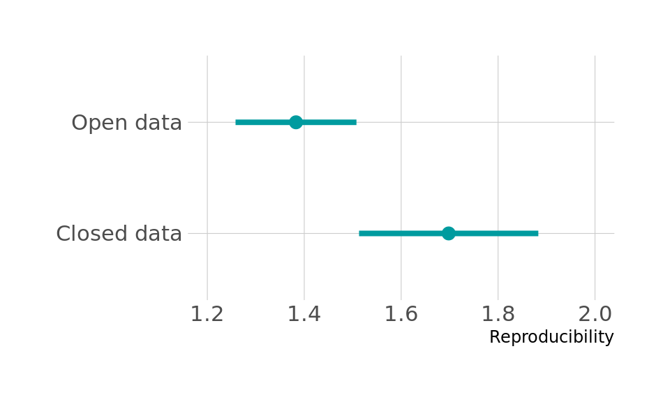
The apparent negative effect is due to the fact that we conditioned on Published, by analysing only the published research. If we condition on a collider, we open that path; in this case we open the path Open data \(\rightarrow\) Published \(\leftarrow\) Rigour \(\rightarrow\) Reproducibility. How conditioning on a collider biases the estimates is difficult to foresee, especially in more complicated cases. In this case, however, there is a reasonably intuitive explanation. In our model, Published depends on both Open data and Rigour (and Novelty, but that is not relevant here): research is more likely to be published in a journal if it has Open data and if it is more rigorous. As a result, research that is published in a journal without Open data tends to have higher Rigour. If research had neither Open data nor sufficiently high Rigour, it would be less likely to be published in a journal at all6. Therefore, published research without Open data has higher Rigour. This higher Rigour in turn affects Reproducibility, leading to higher Reproducibility for published research without Open data.
The example shows how we can draw completely wrong conclusions if we do not use clear causal thinking. Based on the results in Figure 6, some might incorrectly conclude that Open data has a negative causal effect on Reproducibilty. However, in our model, Open data has a positive causal effect on Reproducibility. Hence, we should take great care in interpreting empirical results without causal reflection.
Sometimes, when determining what variables to control for, scholars are inclined to think in terms of ensuring that cases are “comparable”, or to make sure that we compare “like with like”. Although the intuition is understandable, its application is only limited, and at times can be misleading. That is, using the “like with like” intuition, we might be inclined to condition on Published, because we then compare published papers with other published papers. If we do so, we bias the estimation of the causal effect of Open data on Reproducibility, as explained above. In this case, comparing “like with like” may create problems.
Identifying the causal effect
As explained, conditioning on the collider Published opens the non-causal path Open data \(\rightarrow\) Published \(\leftarrow\) Rigour \(\rightarrow\) Reproducibility. This non-causal path is open because Published is open (because it is a collider that is conditioned on), and because Rigour is open (because it is a confounder that is not conditioned on). We can hence close this non-causal path by conditioning on Rigour. In addition, Rigour acts as a confounder on the non-causal path Open data \(\leftarrow\) Rigour \(\rightarrow\) Reproducibility. To identify the causal effect, we hence also need to close this non-causal path by conditioning on Rigour. In short, we close both non-causal paths by conditioning on Rigour.
Panel A in Figure 7 shows the DAG for this question. There are no other non-causal paths that are open, and no causal paths that are closed. The regression model is thus \[\textrm{Reproducibility} \sim \textrm{Open data} + \textrm{Rigour}\] but still restricted to only published research.
Show the code
open_data_effect_on_reproducibility <- get_coefs("open_data", "reproducibility")
# open_data_effect_on_reproducibility

m_od_reprod <- lm(reproducibility ~ open_data + rigour,
                  data = df %>% filter(published == TRUE))
# summary(m_od_reprod)
# coef(m_od_reprod)["open_dataTRUE"]
Show the code
# plot
model_coefs <- tidy(m_od_reprod, conf.int = TRUE) %>%
    mutate(term = case_match(term,
                           "rigour" ~ "Rigour",
                           "open_dataTRUE" ~ "Open Data"))

text_label <- tibble(x = open_data_effect_on_reproducibility,
                     y = "Open Data",
                     label = "True effect")

pal <- colorspace::diverge_hcl(palette = "Tropic", n = 2)
highlight_col <- pal[2]
base_col <- pal[1]

p <- model_coefs %>%
  filter(term != "(Intercept)") %>%
  ggplot() +
  ggdist::geom_pointinterval(aes(estimate, term,
                                 xmin = conf.low, xmax = conf.high), size = 5,
                             colour = base_col) +
  annotate("point", y = "Open Data", x = open_data_effect_on_reproducibility,
           colour = highlight_col, size = 8, shape = "|") +
  geom_text_repel(data = text_label, aes(x = x, y = y, label = label),
                  nudge_x = .2, nudge_y = .2, colour = highlight_col, size = 3) +
  labs(y = NULL, x = "Model estimate") +
  theme_ipsum_rc(grid = "YX", base_size = 10, axis_title_size = 10 ) +
  theme(plot.margin = margin(10, 10, 10, 10)) +
  scale_x_continuous(limits = c(0, 1.5))

# plot both figures
dag_grob <- image_read_pdf(here("causal_intro/article/figures/model_open_data_on_reproducibility.pdf")) %>%
  as.grob()

design <- "
  111##
  111##
  11122
  11122
  111##
  111##
"

wrap_elements(dag_grob) + p +
  plot_layout(design = design) +
  plot_annotation(tag_levels = "A") &
  theme(plot.tag = element_text(size = 15))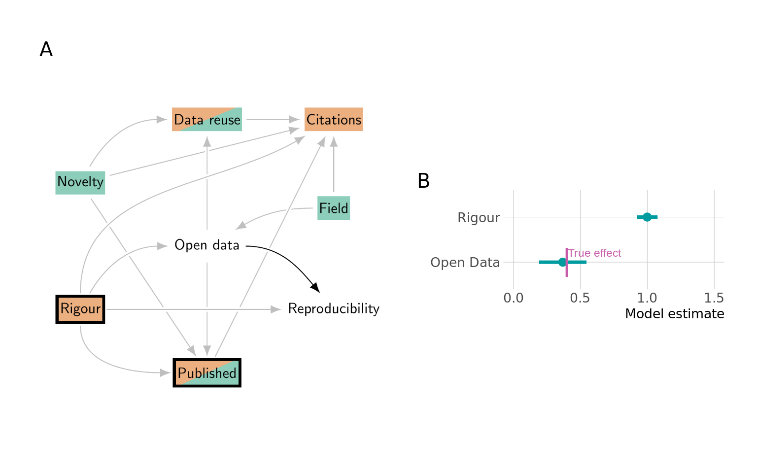
The true effect of Open data on Reproducibility is simply the coefficient of the effect of Open data on Reproducibility that we used in our simulation: it is 0.4 (see Table 1). After controlling for Rigour, our regression model is able to estimate this parameter correctly (panel B of Figure 7), although we are only considering research published in journal articles, therefore “conditioning on a collider”.
The reason we can estimate the parameter correctly is that conditioning on Rigour closes the path Open data \(\rightarrow\) Published \(\leftarrow\) Rigour \(\rightarrow\) Reproducibility. Whether Published is conditioned on is then irrelevant for the identification of the causal effect. If we consider all research instead of only research published in journal articles, our estimates only change minimally.
In identifying the causal effect of Open data on Reproducibility, we do not need to control for other variables, such as Novelty. If there were an additional confounder between Published and Data reuse, this would not change anything in terms of what variables we should control for to identify the effect of Open data on Reproducibility. This shows how making the DAG richer and more nuanced does not necessarily change the identification. Of course, other changes to the DAG do change the identification: if there were another confounder between Open data and Reproducibility, we would need to control for it.
Interpreting regression coefficients and measurement problems
Often, researchers not only interpret the coefficient that is the subject of their main research question, but also interpret the other coefficients. However, it is easy to draw wrong conclusions for those other coefficients, and interpret them incorrectly as causal effects. Since these other effects are often represented in the second table in an article, this was referred to as the “Table 2 fallacy” by Westreich and Greenland (2013).
Let us briefly consider the coefficient for the factor that we controlled for, namely Rigour. We estimated the coefficient for Rigour in our regression model to be about 1. What does this estimate represent? From the point of view of the effect of Rigour on Reproducibility there are two causal paths: one directly from Rigour to Reproducibility and one indirectly, mediated by Open data (we illustrated this earlier in Figure 4). Since we controlled for Open data in our regression model, it means we closed the indirect causal path. All other non-causal paths are also closed, and so there is only one path that is still open, which is the direct causal path from Rigour to Reproducibility. Hence, our estimate of 1 should represent the direct causal effect of Rigour on Reproducibility, and indeed this corresponds with the coefficient we used in our simulation (see again Table 1).
In the example above, we should interpret the estimate of the effect of Rigour on Reproducibility as a direct causal effect, not as a total causal effect. In other cases, coefficients for the controlled factors might not correspond to any causal effect. Indeed, we should carefully reason about any effect we wish to identify, and not interpret any estimates for controlled variables as causal without further reflection.
Additionally, most empirical studies will suffer from measurement problems. That is, the concept of interest is often not observed directly, but measured indirectly through some other proxies or indicators. These issues can be readily incorporated in structural causal models, and might make certain limitations explicit. For example, in the analysis above we controlled for Rigour to infer the causal effect of Open data on Reproducibility, but in reality, we most likely cannot control for Rigour directly. Instead, we are controlling for the measurement of Rigour, for example as measured by expert assessment of the level of rigour. We could include this in the structural causal model as Rigour \(\rightarrow\) Rigour measurement. We cannot directly control for Rigour, and we can only control for Rigour measurement, which does not (fully) close the backdoor path between Open Data and Reproducibility, and might hence still bias the estimate of the causal effect. If Rigour measurement would additionally be affected by other factors, such as Published, this might introduce additional complications. Taking measurement seriously can expose additional challenges that need to be addressed (McElreath 2020, chap. 15).
Discussion
The study of science is a broad field with a variety of methods. Academics have employed a range of perspectives to understand science’s inner workings, driven by the field’s diversity in researchers’ disciplinary backgrounds (Sugimoto et al. 2011; Liu et al. 2023). In this paper we highlight why causal thinking is important for the study of science, in particular for quantitative approaches. In doing so, we do not mean to suggest that we always need to estimate causal effects. Descriptive research is valuable in itself, providing context for uncharted phenomena. Likewise, studies that predict certain outcomes are very useful. However, neither descriptive nor predictive research should be interpreted causally. Both descriptive and predictive work might be able to inform discussions about possible causal mechanisms, and may provide some insight about what might be happening. However, without making causal thinking explicit, they can easily lead to wrong interpretations and conclusions. We covered several related potential issues in data analysis, such as the Table 2 fallacy (see Section 3.3) or the “causal salad” approach (see Section 3.2).
The case for causal thinking
Quantitative research in science studies should make a clear distinction between prediction and causation. For example, if we observe that preregistered studies are more likely to be reproducible, we might use this information to predict which studies are more likely to be reproducible. This might be a perfectly fine predictive model. But is this also a causal effect, where preregistering a study causes the results to be more reproducible? Or is the observed relation between preregistration and reproducibility due to an unobserved confounding factor, such as methodological rigour? Only with an adequate causal model can we try to answer such questions.
The difference between prediction and causation becomes critical when we make policy recommendations. Should research funders mandate open data, in an attempt to improve reproducibility? Besides the problems that such a one-size-fits-all approach might have (Ross-Hellauer et al. 2022), the crucial question is whether or not such an intervention would increase reproducibility. In our DAG, we have assumed that Open data has a moderate but positive effect on Reproducibility. As discussed in Section 3.3, naively analysing the published literature might lead one to incorrectly conclude that Open data is detrimental to Reproducibility. It is therefore imperative that policy recommendations are grounded in careful causal analysis of empirical findings to avoid serious unintended consequences.
More fundamentally, causal thinking is a useful device to connect theories to empirical analyses. Many studies in the social sciences suffer from a vague connection between their theoretical or verbal description and their empirical approach (Yarkoni 2019). A key issue is to translate theoretically derived research questions into estimands (statements about what we aim to estimate), and subsequently, strategies for estimating those estimands (Lundberg, Johnson, and Stewart 2021). In other words, we have to link our statistical models and estimates clearly to our theoretical concepts and research questions (McElreath 2020). Without causal thinking, it is impossible to improve our theoretical understanding of how things work. While building increasingly rich causal diagrams is important in revealing underlying assumptions, this might also reveal deeper problems with our theoretical accounts (Nettle 2023). Deciding on which parts of the system under study to include and which to omit (Smaldino 2023, 318), as well as resisting the urge to add nuance on every turn (Healy 2017), need to accompany any empirical attempt of inferring causality.
Methodologically, structural causal models only make minimal assumptions. If identifying a certain causal effect based on a structural causal model is not possible, stronger assumptions might still allow to identify causal effects. As we have outlined in Section 2, well-known causal inference techniques, such as instrumental variables, difference-in-difference, and regression discontinuity, rely on stronger assumptions, making assumptions about the functional form of the relationships (e.g. linear, or parallel trends), or about thresholds or hurdles. That is the essence of causal inference: we make assumptions to build a causal model, and use these assumptions to argue whether we can identify the causal effect given the observations we make.
Any claims of causal effects derived via causal inference will always depend on the assumptions made. Often, we cannot verify the assumptions empirically, but they might have implications that we can verify empirically. If we find no empirical support for these testable implications, we might need to go back to the drawing board. Finding empirical support for testable implications still does not imply that our assumptions are correct; other assumptions might have similar testable implications. Indeed, we already emphasised this in the context of the DAGs: we cannot say whether a DAG is correct, but we might be able to say whether a DAG is incorrect.
Going beyond—why causal thinking is useful even if causal inference is impossible
In practice, it might not always be possible to estimate a causal effect, because some variables are not observed in a study, or might even be unobservable (Rohrer 2018). We believe that making causal thinking explicit is still highly beneficial to the broader research community in such cases. First, the process of having gone through the exercise of trying to construct a causal model is not wasted, as the model itself might be useful. Researchers might be able to build on the model in subsequent studies, and refine or revise it.
Secondly, causal models make explicit researchers’ beliefs of how specific causal mechanisms work. Other researchers might disagree with those causal models. This is a feature, not a bug. By making disagreement visible, it might be possible to deduce different empirically testable implications, thus advancing the research further, and building a cumulative evidence base.
Thirdly, causal models make explicit why causal estimates might be impossible in a given study. Often, researchers state in their conclusion that there might be missing confounders and that they therefore cannot draw causal conclusions (but they may nonetheless proceed to provide advice that implicitly assumes causality). Simply stating that confounders may exist is not enough. If we, as researchers, believe that we have missed confounders, we should make explicit what we believe we missed. We can of course never be sure that we considered all relevant aspects, but that should not prevent us from trying to be as explicit as possible.
By making explicit how a causal effect is not identifiable, we might be able to suggest variables that we should try to collect in the future. Additionally, by making explicit how our estimates deviate from a causal effect, we might make informed suggestions of the direction of this deviation, e.g. whether we are under- or overestimating the causal effect. Possibly, we might even use some form of sensitivity analysis (Cinelli et al. 2019) to make more informed suggestions.
The social sciences have a distinct advantage over other scientific disciplines when causal inference is challenging: we can talk to people. In case quantitative methods struggle to identify causal relationships, qualitative methods might still provide insight into causal effects, for instance because in interviews people can point out what they believe to be a causal effect. For example, suppose we are interested in the effect of Open data on research efficiency but struggle to quantify the causal effect. We could talk to researchers who have reused openly available datasets, asking whether and how publicly available data has helped them to conduct their research more efficiently. Responses like these might uncover causal evidence where quantitative methods encounter more difficulties.
Finally, developing explicit causal models can benefit qualitative research as well. For example, when developing an interview guide to study a particular phenomenon, it is important to first develop a clear understanding of the potential causal pathways related to that phenomenon. Furthermore, even if qualitative data cannot easily quantify the precise strength of a causal relationship, it may corroborate the structure of a causal model. Ultimately, combining quantitative causal identification strategies with direct qualitative insights on mechanisms can lead to more comprehensive evidence (Munafò and Smith 2018; Tashakkori, Johnson, and Teddlie 2021), strengthening and validating our collective understanding of science.
Acknowledgements
We thank Ludo Waltman, Tony Ross-Hellauer, Jesper W. Schneider and Nicki Lisa Cole for valuable feedback on an earlier version of the manuscript. TK used GPT-4 and Claude v2.1 to assist in language editing during the final revision stage.
Competing interests
The authors have no competing interests.
Funding information
The authors received funding from the European Union’s Horizon Europe framework programme under grant agreement Nos. 101058728 and 101094817. Views and opinions expressed are however those of the authors only and do not necessarily reflect those of the European Union or the European Research Executive Agency. Neither the European Union nor the European Research Executive Agency can be held responsible for them. The Know-Center is funded within COMET—Competence Centers for Excellent Technologies—under the auspices of the Austrian Federal Ministry of Transport, Innovation and Technology, the Austrian Federal Ministry of Economy, Family and Youth and by the State of Styria. COMET is managed by the Austrian Research Promotion Agency FFG.
Data and code availability
All data and code, as well as a reproducible version of the manuscript, are available at (Klebel and Traag 2024).
Theoretical effect of Rigour on Reproducibility
There is a direct effect of Rigour on Reproducibility and a indirect effect, mediated by Open data. Let \(X\) be Rigour, \(Z\) Open Data and \(Y\) Reproducibility. We then have \[X \sim \text{Normal}(0, 1)\] \[Z \sim \text{Bernoulli}(\text{logistic}(\alpha_Z + \beta X + \phi_F))\] \[Y \sim \text{Normal}(\alpha_Y + \gamma X + \theta Z, \sigma)\]
If we try to estimate a simple OLS \(Y = \hat{\alpha} + \hat{\beta}X\), then \[\hat{\beta} = \frac{\text{Cov}(X, Y)}{\text{Var(X)}}.\] Working out \(\text{Cov}(X, Y)\), we can use that \(Y = \alpha_Y + \gamma X + \theta Z + \epsilon_\sigma\) where \(\epsilon_\sigma \sim \text{Normal}(0, \sigma)\), and obtain that \[\text{Cov}(X, Y) = \gamma \text{Cov}(X, X) + \theta \text{Cov}(X, Z) + \text{Cov}(X, \epsilon_\sigma),\] where \(\text{Cov}(X,X) = \text{Var}(X, X) = 1^2 = 1\) and \(\text{Cov}(X, \epsilon_\sigma) = 0\), because \(\epsilon_\sigma\) is independent of \(X\). Hence, we obtain \[\text{Cov}(X, Y) = \gamma + \theta \text{Cov}(X, Z).\] Writing out \(\text{Cov}(X, Z)\), we find that \(\text{Cov}(X, Z) = E(X Z)\) because \(E(X) = 0\). Then elaborating \(E(X Z) = E(E(X Z | F))\), we can expand \(E(X Z | F)\) as a sum \[E(X Z | F) = \int_x \sum_{z=0}^1 x z P(Z = z \mid X = x, F) P(X = x) \mathrm{d}x\] Obviously, \(x z = 0\) when \(z = 0\), while \(x z = x\) when \(z = 1\). Hence, this simplifies to only the \(z = 1\) part, such that \[E(X Z | F) = \int_x x P(Z = 1 \mid X = x, F) P(X = x) \mathrm{d}x\] or \[E(X Z \mid F) = \int_x x \cdot \text{logistic}(\alpha_Z + \beta x + \phi_F) \cdot f(x) \mathrm{d}x,\] where \(f(x)\) is the pdf of \(X \sim \text{Normal}(0,1)\). Unfortunately, this does not seem to have an analytical solution, so we numerically integrate this.
The total causal effect of Rigour on Reproducibility is very close to the direct causal effect of Rigour on Reproducibility (which is 1), because the indirect effect via Rigour \(\rightarrow\) Open data is small.
Theoretical effect of Open data on citations
There are two causal paths of the effect of Open data on Citations. The first causal path is mediated by Data reuse and the second is mediated by Published. Let \(X\) be Open data, \(Y\) be Citations, \(D\) be Data reuse and \(P\) be Published. Since we use a normal distribution for Citations we can simply write \[E(Y) = \alpha + \beta_{DY} D + \beta_{PY} P + \beta_{\text{novelty,Y}} \cdot \textit{Novelty} + \beta_{\text{rigour,Y}} \cdot \textit{Rigour} + \beta_{\text{field,Y}} \cdot \textit{Field},\] where we can consider Field a dummy variable, representing the effect of field 2 relative to field 1 (i.e. field 1 is the reference category).
The change in \(Y\), i.e. \(\Delta Y\), relative to changing \(X\), i.e. \(\Delta X\), from \(0\) to \(1\) is then \[ \frac{\Delta Y(X)}{\Delta X} =
\beta_{DY} \frac{\Delta D(X)}{\Delta X} +
\beta_{PY} \frac{\Delta P(X)}{\Delta X}
\] The first part is simple, since \(D\) is a normal distribution, yielding \(\frac{\Delta D(X)}{\Delta X} = \beta_{XD}\). The second part is more convoluted, since \(P\) is a logistic distribution of a normal variable. For that reason, we calculate \(\frac{\Delta P(X)}{\Delta X}\) numerically using logitnorm::momentsLogitnorm (version 0.8.38) in R.
Validation of argument against stepwise regression
In Section 3.2, we claimed that stepwise regression would suggest to include the mediating variables Published and Open data and to remove Open Data from the regression model. The output below demonstrates this behaviour.
We first start with a full model that includes all variables.
Show the code
full_model <- lm(citations ~ ., data = df)Next, we let R select variables in a stepwise fashion, considering both directions (including or excluding variables) at each step.
Show the code
step_model <- MASS::stepAIC(full_model, direction = "both", trace = TRUE)Start: AIC=14.39
citations ~ rigour + novelty + field + open_data + published +
data_reuse + reproducibility
Df Sum of Sq RSS AIC
- reproducibility 1 0.0 998.4 12.42
- open_data 1 0.2 998.6 12.59
<none> 998.4 14.39
- published 1 407.8 1406.2 354.90
- rigour 1 1683.9 2682.2 1000.65
- novelty 1 1946.4 2944.7 1094.02
- data_reuse 1 3620.3 4618.7 1544.10
- field 1 10158.0 11156.4 2426.01
Step: AIC=12.42
citations ~ rigour + novelty + field + open_data + published +
data_reuse
Df Sum of Sq RSS AIC
- open_data 1 0.2 998.6 10.61
<none> 998.4 12.42
+ reproducibility 1 0.0 998.4 14.39
- published 1 407.8 1406.3 352.94
- novelty 1 1946.4 2944.9 1092.06
- rigour 1 3199.3 4197.7 1446.55
- data_reuse 1 3623.4 4621.8 1542.79
- field 1 10171.5 11170.0 2425.23
Step: AIC=10.61
citations ~ rigour + novelty + field + published + data_reuse
Df Sum of Sq RSS AIC
<none> 998.6 10.61
+ open_data 1 0.2 998.4 12.42
+ reproducibility 1 0.0 998.6 12.59
- published 1 505.6 1504.2 418.26
- novelty 1 2394.6 3393.2 1231.78
- rigour 1 3281.9 4280.5 1464.06
- data_reuse 1 4743.2 5741.9 1757.78
- field 1 14922.0 15920.6 2777.61We can see that the algorithm first removes Open data, and then Reproducibility. The final model is then as follows:
Show the code
summary(step_model)
Call:
lm(formula = citations ~ rigour + novelty + field + published +
    data_reuse, data = df)

Residuals:
     Min       1Q   Median       3Q      Max
-3.08249 -0.68542 -0.01525  0.70217  3.02677

Coefficients:
              Estimate Std. Error t value Pr(>|t|)
(Intercept)   -1.26727    0.11955  -10.60   <2e-16 ***
rigour         1.92751    0.03372   57.16   <2e-16 ***
novelty        2.01798    0.04133   48.82   <2e-16 ***
field         10.11475    0.08299  121.87   <2e-16 ***
publishedTRUE  2.06206    0.09192   22.43   <2e-16 ***
data_reuse     1.95682    0.02848   68.71   <2e-16 ***
---
Signif. codes:  0 '***' 0.001 '**' 0.01 '*' 0.05 '.' 0.1 ' ' 1

Residual standard error: 1.002 on 994 degrees of freedom
Multiple R-squared:  0.9878,    Adjusted R-squared:  0.9878
F-statistic: 1.616e+04 on 5 and 994 DF,  p-value: < 2.2e-16
The case against causal salad
Table 2 illustrates the result of the ‘causal salad’ approach of including all variables. Because this model controls for mediators, the effect of Open data on Citations appears to be zero. The researcher could thus be led to conclude that Open data has no effect on Citations, which is incorrect.
Show the code
coef_val <- round(coef(m_od_citations)[["open_dataTRUE"]], 2)

caption <- paste0(
  'Example of "causal salad". The "Correct model" to estimate the causal effect of *Open data* on *Citations* identifies the effect to be ', coef_val, '. If the researcher were to include all variables, it might seem as if there was no effect of *Open data* on *Citations*. Values in brackets show p-values.'
)
Show the code
named_models <- list("Correct model" = m_od_citations,
                     "'Causal salad' model" = full_model)

coef_names <- c("(Intercept)" = "Intercept",
                "open_dataTRUE" = "Open Data",
                "field" = "Field", "rigour" = "Rigour",
                "novelty" = "Novelty",
                "data_reuse" = "Data reuse",
                "publishedTRUE" = "Published",
                "reproducibility" = "Reproducibility")

modelsummary(named_models, output = "flextable", statistic = "p.value",
             gof_omit = 'IC|Log|Adj|RMSE', coef_map = coef_names) %>%
  align(align = "center", part = "all") %>%
  bg(i = 3:4, j = 2, bg = "grey90") %>%
  bg(i = 3:4, j = 3, bg = "coral1") %>%
  autofit(add_w = .1)
| Correct model | 'Causal salad' model |
|---|---|---|
Intercept | -2.519 | -1.295 |
(<0.001) | (<0.001) | |
Open Data | 5.294 | -0.061 |
(<0.001) | (0.655) | |
Field | 10.213 | 10.140 |
(<0.001) | (<0.001) | |
Rigour | 2.355 | 1.919 |
(<0.001) | (<0.001) | |
Novelty | 2.010 | |
(<0.001) | ||
Data reuse | 1.964 | |
(<0.001) | ||
Published | 2.082 | |
(<0.001) | ||
Reproducibility | 0.006 | |
(0.849) | ||
Num.Obs. | 1000 | 1000 |
R2 | 0.726 | 0.988 |
References
Aagaard, Kaare, and Jesper W Schneider. 2017. “Some Considerations about Causes and Effects in Studies of Performance-Based Research Funding Systems.” J. Informetr. 11 (3): 923–26. https://doi.org/10.1016/j.joi.2017.05.018.
Arif, Suchinta, and M. Aaron MacNeil. 2023. “Applying the Structural Causal Model Framework for Observational Causal Inference in Ecology.” Ecological Monographs 93 (1): e1554. https://doi.org/10.1002/ecm.1554.
Balke, Alexander, and Judea Pearl. 2012. “Bounds on Treatment Effects from Studies with Imperfect Compliance.” Journal of the American Statistical Association, February. https://www.tandfonline.com/doi/abs/10.1080/01621459.1997.10474074.
Cinelli, Carlos, Daniel Kumor, Bryant Chen, Judea Pearl, and Elias Bareinboim. 2019. “Sensitivity Analysis of Linear Structural Causal Models.” In Proceedings of the 36th International Conference on Machine Learning, 1252–61. PMLR. https://proceedings.mlr.press/v97/cinelli19a.html.
Cunningham, Scott. 2021. Causal Inference. Yale University Press.
Davis, Philip M. 2020. “Reanalysis of Tweeting Study Yields No Citation Benefit.” The Scholarly Kitchen. https://scholarlykitchen.sspnet.org/2020/07/13/tweeting-study-yields-no-benefit/.
Davis, Philip M, Bruce V Lewenstein, Daniel H Simon, James G Booth, and Mathew J L Connolly. 2008. “Open Access Publishing, Article Downloads, and Citations: Randomised Controlled Trial.” BMJ 337 (7665): 343–45. https://doi.org/10.1136/bmj.a568.
Deffner, Dominik, Julia M. Rohrer, and Richard McElreath. 2022. “A Causal Framework for Cross-Cultural Generalizability.” Advances in Methods and Practices in Psychological Science 5 (3): 25152459221106366. https://doi.org/10.1177/25152459221106366.
Dong, Xianlei, Jiahui Xu, Yi Bu, Chenwei Zhang, Ying Ding, Beibei Hu, and Yang Ding. 2022. “Beyond Correlation: Towards Matching Strategy for Causal Inference in Information Science.” Journal of Information Science 48 (6): 735–48. https://doi.org/10.1177/0165551520979868.
Elwert, Felix. 2013. “Graphical Causal Models.” In, edited by Stephen L. Morgan, 245–73. Handbooks of Sociology and Social Research. Dordrecht: Springer Netherlands. https://doi.org/10.1007/978-94-007-6094-3_13.
Fecher, Benedikt, and Sascha Friesike. 2014. “Open Science: One Term, Five Schools of Thought.” In, edited by Sönke Bartling and Sascha Friesike, 17–47. Cham: Springer International Publishing. https://doi.org/10.1007/978-3-319-00026-8_2.
Gläser, Jochen, and Grit Laudel. 2016. “Governing Science: How Science Policy Shapes Research Content.” European Journal of Sociology 57 (1): 117–68. https://doi.org/10.1017/S0003975616000047.
Goodman, Steven N., Jesse Berlin, Suzanne W. Fletcher, and Robert H. Fletcher. 1994. “Manuscript Quality Before and After Peer Review and Editing at Annals of Internal Medicine.” Annals of Internal Medicine 121 (1): 11–21. https://doi.org/10.7326/0003-4819-121-1-199407010-00003.
Hardwicke, Tom E., Manuel Bohn, Kyle MacDonald, Emily Hembacher, Michèle B. Nuijten, Benjamin N. Peloquin, Benjamin E. deMayo, Bria Long, Erica J. Yoon, and Michael C. Frank. 2021. “Analytic Reproducibility in Articles Receiving Open Data Badges at the Journal Psychological Science: An Observational Study.” Royal Society Open Science 8 (1): 201494. https://doi.org/10.1098/rsos.201494.
Hardwicke, Tom E., Maya B. Mathur, Kyle MacDonald, Gustav Nilsonne, George C. Banks, Mallory C. Kidwell, Alicia Hofelich Mohr, et al. 2018. “Data Availability, Reusability, and Analytic Reproducibility: Evaluating the Impact of a Mandatory Open Data Policy at the Journal Cognition.” Royal Society Open Science 5 (8): 180448. https://doi.org/10.1098/rsos.180448.
Healy, Kieran. 2017. “Fuck Nuance.” Sociological Theory 35 (2): 118–27. https://doi.org/10.1177/0735275117709046.
Hünermund, Paul, and Elias Bareinboim. 2023. “Causal Inference and Data Fusion in Econometrics.” arXiv. https://doi.org/10.48550/arXiv.1912.09104.
Huntington-Klein, Nick. 2021. The Effect: An Introduction to Research Design and Causality. CRC Press.
Klebel, Thomas, Nicki Lisa Cole, Lena Tsipouri, Eva Kormann, Istvan Karasz, Sofia Liarti, Lennart Stoy, Vincent Traag, Silvia Vignetti, and Tony Ross-Hellauer. 2023. “PathOS - D1.2 Scoping Review of Open Science Impact,” May. https://zenodo.org/record/7883699.
Klebel, Thomas, and Vincent Traag. 2024. “Code for "Introduction to Causality in Science Studies".” Zenodo. https://doi.org/10.5281/zenodo.10639143.
Kwon, Seokbeom, and Kazuyuki Motohashi. 2021. “Incentive or Disincentive for Research Data Disclosure? A Large-Scale Empirical Analysis and Implications for Open Science Policy.” International Journal of Information Management 60 (October): 102371. https://doi.org/10.1016/j.ijinfomgt.2021.102371.
Liu, Lu, Benjamin F. Jones, Brian Uzzi, and Dashun Wang. 2023. “Data, Measurement and Empirical Methods in the Science of Science.” Nature Human Behaviour 7 (7): 1046–58. https://doi.org/10.1038/s41562-023-01562-4.
Luc, Jessica G. Y., Michael A. Archer, Rakesh C. Arora, Edward M. Bender, Arie Blitz, David T. Cooke, Tamara Ni Hlci, et al. 2021. “Does Tweeting Improve Citations? One-Year Results From the TSSMN Prospective Randomized Trial.” The Annals of Thoracic Surgery 111 (1): 296–300. https://doi.org/10.1016/j.athoracsur.2020.04.065.
Lundberg, Ian, Rebecca Johnson, and Brandon M. Stewart. 2021. “What Is Your Estimand? Defining the Target Quantity Connects Statistical Evidence to Theory.” American Sociological Review 86 (3): 532–65. https://doi.org/10.1177/00031224211004187.
Malmgren, R. Dean, Julio M. Ottino, and Luís A. Nunes Amaral. 2010. “The Role of Mentorship in Protégé Performance.” Nature 465 (7298): 622–26. https://doi.org/10.1038/nature09040.
McElreath, Richard. 2020. Statistical Rethinking: A Bayesian Course with Examples in r and Stan. 2nd ed. CRC Texts in Statistical Science. Boca Raton: Taylor; Francis, CRC Press.
Molloy, Jennifer C. 2011. “The Open Knowledge Foundation: Open Data Means Better Science.” PLoS Biology 9 (12): e1001195. https://doi.org/10.1371/journal.pbio.1001195.
Munafò, Marcus R., and George Davey Smith. 2018. “Robust Research Needs Many Lines of Evidence.” Nature 553 (7689): 399–401. https://doi.org/10.1038/d41586-018-01023-3.
Nettle, Author Daniel. 2023. “It Probably Is That Bad.” https://www.danielnettle.org.uk/2023/11/09/it-probably-is-that-bad/.
Nosek, Brian A., Tom E. Hardwicke, Hannah Moshontz, Aurélien Allard, Katherine S. Corker, Anna Dreber, Fiona Fidler, et al. 2022. “Replicability, Robustness, and Reproducibility in Psychological Science.” Annual Review of Psychology 73 (1): 719–48. https://doi.org/10.1146/annurev-psych-020821-114157.
Nuijten, Michèle B., Jeroen Borghuis, Coosje L. S. Veldkamp, Linda Dominguez-Alvarez, Marcel A. L. M. van Assen, and Jelte M. Wicherts. 2017. “Journal Data Sharing Policies and Statistical Reporting Inconsistencies in Psychology.” Edited by Simine Vazire and Chris Chambers. Collabra: Psychology 3 (1): 31. https://doi.org/10.1525/collabra.102.
Pearl, Judea. 2009. Causality: Models, Reasoning, and Inference. 2nd ed. Cambridge University Press. https://doi.org/10.1017/CBO9780511803161.
Piwowar, Heather, Roger Day, and Douglas Fridsma. 2007. “Sharing Detailed Research Data Is Associated with Increased Citation Rate.” Edited by John Ioannidis. PLoS ONE 2 (3): e308. https://doi.org/10.1371/journal.pone.0000308.
Piwowar, Heather, and Todd J. Vision. 2013. “Data Reuse and the Open Data Citation Advantage.” https://doi.org/10.7287/peerj.preprints.1v1.
Rohrer, Julia M. 2018. “Thinking Clearly about Correlations and Causation: Graphical Causal Models for Observational Data.” Advances in Methods and Practices in Psychological Science 1 (1): 27–42. https://doi.org/10.1177/2515245917745629.
Rohrer, Julia M., Paul Hünermund, Ruben C. Arslan, and Malte Elson. 2022. “That’s a Lot to Process! Pitfalls of Popular Path Models.” Advances in Methods and Practices in Psychological Science 5 (2): 25152459221095827. https://doi.org/10.1177/25152459221095827.
Ross-Hellauer, Tony, Thomas Klebel, Alexandra Bannach-Brown, Serge P. J. M. Horbach, Hajira Jabeen, Natalia Manola, Teodor Metodiev, et al. 2022. “TIER2: Enhancing Trust, Integrity and Efficiency in Research Through Next-Level Reproducibility.” Research Ideas and Outcomes 8 (December): e98457. https://doi.org/10.3897/rio.8.e98457.
Smaldino, Paul E. 2023. Modeling Social Behavior: Mathematical and Agent-Based Models of Social Dynamics and Cultural Evolution. Princeton: Princeton University Press.
Sugimoto, Cassidy R., Chaoqun Ni, Terrell G. Russell, and Brenna Bychowski. 2011. “Academic Genealogy as an Indicator of Interdisciplinarity: An Examination of Dissertation Networks in Library and Information Science.” Journal of the American Society for Information Science and Technology 62 (9): 1808–28. https://doi.org/10.1002/asi.21568.
Tashakkori, Abbas, R. Burke Johnson, and Charles Teddlie. 2021. Foundations of Mixed Methods Research: Integrating Quantitative and Qualitative Approaches in the Social and Behavioral Sciences. Second edition. Los Angeles London New Delhi Singapore Washington DC Melbourne: SAGE.
Tennant, Jonathan P., François Waldner, Damien C. Jacques, Paola Masuzzo, Lauren B. Collister, and Chris H. J. Hartgerink. 2016. “The Academic, Economic and Societal Impacts of Open Access: An Evidence-Based Review,” September. https://doi.org/10.12688/f1000research.8460.3.
Tomkins, Andrew, Min Zhang, and William D Heavlin. 2017. “Reviewer Bias in Single- Versus Double-Blind Peer Review.” Proc. Natl. Acad. Sci. U. S. A. 114 (48): 12708–13. https://doi.org/10.1073/pnas.1707323114.
Traag, V. A., and L. Waltman. 2022. “Causal Foundations of Bias, Disparity and Fairness.” arXiv. https://doi.org/10.48550/arXiv.2207.13665.
Waltman, Ludo, and Nees Jan van Eck. 2019. “Field Normalization of Scientometric Indicators.” Springer Handbook of Science and Technology Indicators, 281–300. https://doi.org/10.1007/978-3-030-02511-3_11.
Westreich, Daniel, and Sander Greenland. 2013. “The Table 2 Fallacy: Presenting and Interpreting Confounder and Modifier Coefficients.” American Journal of Epidemiology 177 (4): 292–98. https://doi.org/10.1093/aje/kws412.
Woods, Helen Buckley, and Stephen Pinfield. 2022. “Incentivising Research Data Sharing: A Scoping Review.” Wellcome Open Research 6 (April): 355. https://doi.org/10.12688/wellcomeopenres.17286.2.
Yarkoni, Tal. 2019. “The Generalizability Crisis,” November. https://doi.org/10.31234/osf.io/jqw35.
Footnotes
Depending on the functional specification, \(Y\) might only change in specific circumstances. For example, suppose our functional specification includes a hurdle, such that \[Y = f(X,Z) = \begin{cases} 0 & \text{if~} 0 < X < 5, \\ Z^2 & \text{if~} X \geq 5. \\ \end{cases}\] In this case, only a change in \(X\) that crosses the threshold of 5 results in a change in \(Y\); anything else will not change \(Y\). A more precise formulation therefore is that if \(X\) is not a parent of \(Y\) (nor a further ancestor) then changes in \(X\) never lead to changes in \(Y\). This also makes clear that leaving out a link in a DAG is a stronger assumption than keeping a link in. A link that is present in a DAG indicates that there might be some dependency. A link that is absent indicates that there is no (direct) dependency at all.↩︎
In technical terms, two variables \(X\) and \(Y\) that are not correlated are said to be \(d\)-separated, sometimes denoted by \(X \perp Y\). Two variables \(X\) and \(Y\) that are correlated are said to be \(d\)-connected, sometimes denoted by \(X \not\perp Y\). Whether two variables \(X\) and \(Y\) are \(d\)-separated or \(d\)-connected depends on whether other variables \(\mathcal{Z} = Z_1, Z_2, \ldots\) are controlled for or not. If two variables \(X\) and \(Y\) are \(d\)-separated, conditional on controlling for variables \(\mathcal{Z}\), this is denoted as \(X \perp Y \mid \mathcal{Z}\). We do not use this notation here, but you might encounter the notation in other texts.↩︎
Note that there are many additional paths in this example: Open data \(\leftarrow\) Rigour \(\rightarrow\) Citations, Open data \(\rightarrow\) Reproducibility \(\leftarrow\) Rigour \(\rightarrow\) Citations, etc.↩︎
In this case, our assumed DAG implies that there should be no causal effect of Reproducibility on Citations. If we condition on Open data and Rigour all non-causal paths are closed, meaning that we then expect to find no correlation. If, in contrast, we still find a non-zero correlation after conditioning on Open data and Rigour, it means our DAG is incorrect, and we need to revise it.↩︎
We will write the equation in the typical style of R. For example, \(Y \sim X + A\), refers to the linear equation \(Y = \alpha + \beta_X X + \beta_A A\), where we are interested in estimating the coefficients \(\alpha\), \(\beta_X\) and \(\beta_A\).↩︎
In our DAG, Published is also affected by Novelty, and the same reasoning applies there. In this case, research that is published in a journal, but that does not share Open data and has low Rigour, is then more likely to have high Novelty. Otherwise, it again would most likely not have been published in a journal at all.↩︎
Reuse
Open Science Indicator Handbook © 2024 by PathOS is licensed under CC BY 4.0
(View License)
Citation
BibTeX citation:
@online{apartis2023,
  author = {Apartis, S. and Catalano, G. and Consiglio, G. and Costas,
    R. and Delugas, E. and Dulong de Rosnay, M. and Grypari, I. and
    Karasz, I. and Klebel, Thomas and Kormann, E. and Manola, N. and
    Papageorgiou, H. and Seminaroti, E. and Stavropoulos, P. and Stoy,
    L. and Traag, V.A. and van Leeuwen, T. and Venturini, T. and
    Vignetti, S. and Waltman, L. and Willemse, T.},
  title = {PathOS - {D2.1} - {D2.2} - {Open} {Science} {Indicator}
    {Handbook}},
  date = {2023},
  url = {https://handbook.pathos-project.eu/causal_intro/article/intro-causality.html},
  doi = {10.5281/zenodo.8305626},
  langid = {en}
}
For attribution, please cite this work as:
Apartis, S., G. Catalano, G. Consiglio, R. Costas, E. Delugas, M. Dulong
de Rosnay, I. Grypari, et al. 2023. “PathOS - D2.1 - D2.2 - Open
Science Indicator Handbook.” Zenodo. 2023. https://doi.org/10.5281/zenodo.8305626.